Swift
Source: https://www.nature.com/articles/s41586-023-06419-4
Abstract
First-person perspective (FPV) drone racing is a televised sport in which professional competitors pilot high-speed aircraft across a 3D track. Each pilot observes the surrounding environment from the drone's perspective using video feeds from an onboard camera. Achieving the level of autonomous drone control achieved by professional pilots is challenging because the robot needs to fly within limits while estimating its speed and position on the track using only onboard sensors[^1]. Here we present Swift, an autonomous system that can race against human world champion-level physical vehicles. The system combines deep reinforcement learning (RL) in simulation with data collected in the real world. Swift competed in real-world head-to-head races against three human champions, including two world champions from international leagues. Swift won several races against each human champion and set the fastest race time. This work represents a milestone in mobile robotics and machine intelligence[^2] and may inspire the deployment of hybrid learning-based solutions in other physical systems.
Main
Deep reinforcement learning [^3] has driven some of the recent advances in artificial intelligence. Policies trained using deep reinforcement learning have outperformed humans in complex competitive games, including Atari 4, 5, 6 , Go 5, 7, 8, 9 , Chess 5 , 9, StarCraft [^10] , Dota 2 ( Ref. [^11] ) , and Gran Turismo 12, 13. These impressive demonstrations of machine intelligence have been primarily limited to simulations and board game environments that allow for policy search in precisely replicated test conditions. Overcoming this limitation and demonstrating championship-level performance in competitive sports is a long - standing problem in autonomous mobile robotics and artificial intelligence 14, 15, 16.
FPV drone racing is a televised sport in which highly trained human pilots push aircraft to their physical limits through high-speed, agile maneuvers (Figure 1a ). The aircraft used in FPV racing are quadcopters, which are among the most agile machines ever created (Figure 1b ). During competition, the aircraft exert forces exceeding five times their own weight or more, reaching speeds exceeding 100 km h⁻¹ and accelerations several times greater than gravity, even in confined spaces. Each aircraft is remotely controlled by a human pilot wearing a headset that displays a video stream from an onboard camera, creating an immersive "first-person perspective" experience (Figure 1c ).
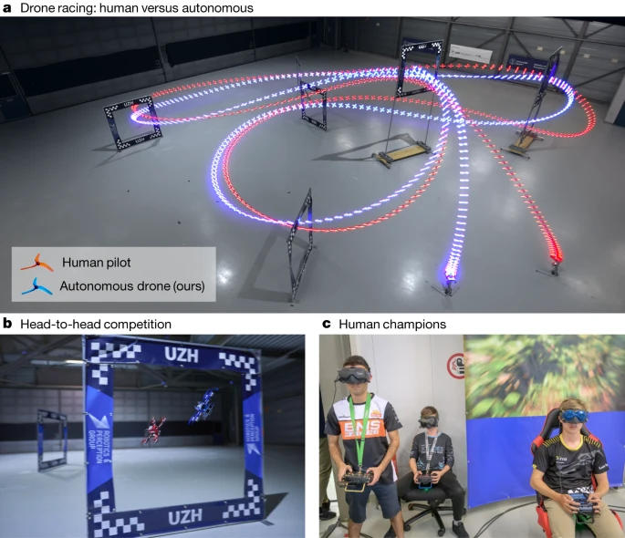
Figure 1: Drone racing.
Attempts to create autonomous systems that can match the performance of human pilots can be traced back to the first autonomous drone race in 2016 (Ref. [^17] ). A series of innovations followed, including using deep networks to identify the next gate location, 18,19,20 transferring race strategies from simulation to reality ,21,22 and accounting for uncertainty in perception, 23,24. The 2019 AlphaPilot autonomous drone race showcased some of the best research in this area.25 However, the top two teams still took almost twice as long as professional human pilots to complete the course.26,27 More recently , autonomous systems have begun to match the performance of human experts.28,29,30 However, these efforts rely on near- perfect state estimates provided by external motion capture systems. This makes comparisons with human pilots unfair, as humans only have access to onboard observations from the drone.
This paper introduces Swift, an autonomous flight system that can fly a quadrotor in a competition against a human world champion using only onboard sensors and computational power. Swift consists of two key modules: (1) a perception system that converts high-dimensional visual and inertial information into low-dimensional representations; and (2) a control policy that takes the low-dimensional representations generated by the perception system and generates control commands.
The control policy is represented by a feedforward neural network and trained in simulation using model-free on-policy deep reinforcement learning [^31]. To bridge the gap between the simulation and the physical world in terms of perception and dynamics, we utilize non-parametric empirical noise models estimated from data collected from the physical system. These empirical noise models have been shown to be crucial for successfully transferring control policies from simulation to the real world.
We evaluated Swift on a physical track designed by professional drone racing pilots (Figure 1a ). The track consisted of seven square gates measuring 30 × 30 × 8 meters, forming a 75-meter lap. Swift competed against three human champions on this track: 2019 Drone Racing League World Champion Alex Vanover, two-time MultiGP International Open World Cup champion Thomas Bitmatta, and three-time Swiss National Champion Marvin Schaepper. The quadrotors used by Swift and the human pilots had the same weight, shape, and propulsion. They are similar to drones used in international competitions.
The human pilots practiced on the track for a week. Afterward, each pilot competed in several head-to-head races against Swift (Figures 1a, b ). In each head-to-head race, two drones (one controlled by a human pilot and one by Swift) started from the podium. The race began with an acoustic signal. The first drone to complete three full laps of the track, passing through all gates in the correct order on each lap, won the race.
Swift defeated every human pilot in the competition and set the fastest time in the event. To our knowledge, this is the first time an autonomous mobile robot has achieved world championship-level performance in a real-world competitive sport.
Swift
Swift combines learning-based and traditional algorithms to map onboard sensor readings to control commands. This mapping consists of two parts: (1) an observation strategy, which distills high-dimensional visual and inertial information into a task-specific, low-dimensional encoding; and (2) a control strategy, which converts the encoding into instructions for the drone. A schematic diagram of the system is shown in Figure 2.
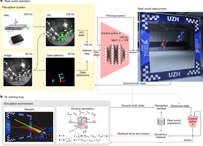
Figure 2: Swift system.
The observation policy consists of a visual-inertial estimator 32, 33, which operates in conjunction with a gate detector 26, a convolutional neural network that detects race gates in the onboard imagery. The detected gates are then used to estimate the drone's global position and orientation along the track. This is done using a camera resection algorithm [^34] in conjunction with the track map. The global pose estimate obtained from the gate detector is then combined with the estimate from the visual-inertial estimator via a Kalman filter to more accurately represent the robot's state. The control policy is represented by a two-layer perceptron that maps the output of the Kalman filter to control commands for the drone. The policy is trained in simulation using policy-based model-free deep reinforcement learning 31. During training, the policy maximizes the reward for approaching the next race gate [^35] combined with the perceptual goal of keeping the next gate within the camera's field of view. Seeing the next gate is rewarded because it increases the accuracy of the pose estimate.
Optimizing a policy solely through simulation can lead to poor performance on physical hardware if the discrepancies between simulation and reality are not eliminated. These discrepancies are primarily due to two factors: (1) the difference between simulated and real-world dynamics, and (2) the noisy estimate of the robot state made by the observation policy when fed real-world sensor data. We mitigate these discrepancies by collecting a small amount of real-world data and leveraging this data to improve the realism of the simulator.
Specifically, as the UAV drives around the track, we record observations from the robot’s onboard sensors along with high-precision pose estimates from a motion capture system. During this data collection phase, the robot is controlled by a policy trained in simulation that operates on the pose estimates provided by the motion capture system. The recorded data allows the identification of characteristic failure modes in perception and dynamics observed through the track. The complexity of these perception failures and unmodeled dynamics depends on the environment, platform, track, and sensors. Perception and dynamic residuals are modeled using Gaussian processes [^36] and k- nearest neighbor regression, respectively. This choice is motivated by our empirical finding that perception residuals are stochastic, while dynamic residuals are largely deterministic (Extended Data Fig. 1 ). These residual models are integrated into the simulation, and the racing policy is fine-tuned in this augmented simulation. This approach is related to the empirical actuator model used for simulation-to-reality transfer in Ref. [^37] but goes further by incorporating empirical modeling of the perception system and accounting for the stochastic nature of the platform state estimates.
We eliminated each component of Swift in controlled experiments reported in the Extended Data. Furthermore, we compared it with recent work using traditional methods, including trajectory planning and model predictive control (MPC), to solve autonomous drone racing tasks. While such methods achieve comparable or even superior performance to ours under ideal conditions (such as simplified dynamics and perfect knowledge of the robot's state), their performance collapses when their assumptions are violated. We found that methods that rely on precomputed paths28 , 29 are particularly sensitive to noisy perception and dynamics. Even equipped with high-precision state estimates from motion capture systems, traditional methods fail to achieve lap times competitive with Swift or human world champions. Detailed analysis is provided in the Extended Data.
Results
Drone races are conducted on courses designed by external, world-class FPV pilots. These courses are filled with unique maneuvers and challenges, such as the Split-S (Figure 1a (top right) and Figure 4d ). Even in the event of a collision, pilots can continue the race, provided their drones are still able to fly. If both drones collide and are unable to complete the race, the drone that travels further on the course wins.
As shown in Figure 3b, Swift won 5 of 9 races against A. Vanover, 4 of 7 against T. Bitmatta, and 6 of 9 against M. Schaepper. Of Swift's 10 losses, 40% were due to collisions with opponents, 40% were due to collisions with gates, and 20% were due to the drone being slower than the human pilot. Overall, Swift won every race against the human pilot. Swift also set the fastest time, beating the best time by a human pilot (A. Vanover) by half a second.
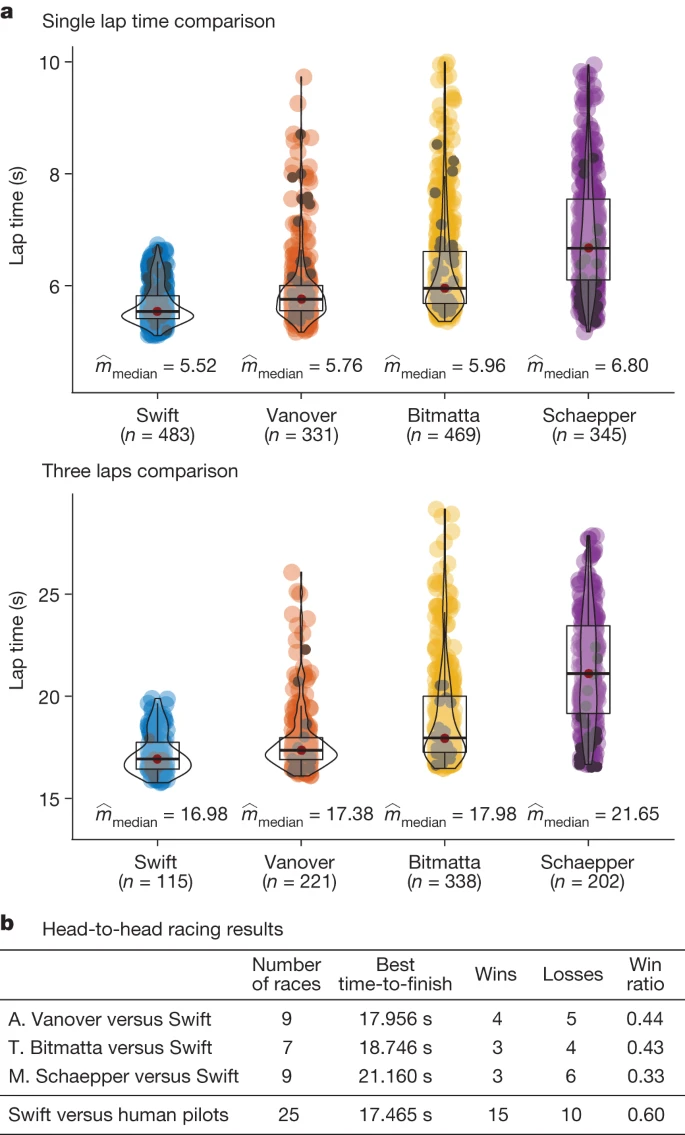
Figure 3: Results.
Figure 4 and Extended Data Table 1d analyze the fastest laps flown by Swift and each human pilot. Although Swift was faster overall than all human pilots, it was not faster on all individual sections of the track (Extended Data Table 1 ). Swift was consistently faster at the start and in tight turns, such as the forked S. At the start, Swift had a shorter reaction time, starting 120 milliseconds earlier than the human pilots on average. Furthermore, it accelerated faster, reaching a higher speed when entering the first gate (Extended Data Table 1d, segment 1). In tight turns, as shown in Figures 4c and 4d, Swift was able to find more compact maneuvers. One hypothesis is that Swift optimizes its trajectory over longer timescales than the human pilots. Model-free RL is known to optimize long-term rewards via a value function [^38]. In contrast, human pilots plan their movements over shorter timescales, at most one gate ahead [^39]. This is evident , for example, in segment S (Figure 4b, d ), where the human pilot was faster at the beginning and end of the maneuver but slower overall (Extended Data Table 1d, segment 3). Furthermore, the human pilot maneuvered the aircraft toward the next gate earlier than Swift (Figure 4c, d ). We believe that the human pilot was accustomed to keeping the upcoming gate in view, while Swift had learned to rely on other cues for certain maneuvers, such as inertial data and visual odometry for features in the surrounding environment. Overall, averaged across the entire course, the autonomous drone achieved the highest average speed, found the shortest course, and managed to keep the aircraft closer to its driving limit throughout the race, as shown by average thrust and power (Extended Data Table 1d ).
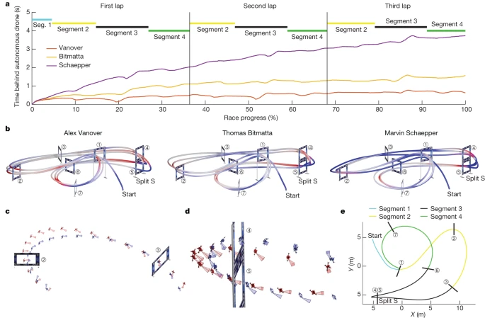
Figure 4: Analysis.
We also compared Swift's performance with that of a human champion in a time trial (Figure 3a ). In a time trial, a single pilot races around a track, completing laps at the pilot's discretion. We accumulated time trial data from practice weeks and races, including training runs (Figure 3a, color) and laps flown under race conditions (Figure 3a, black). For each competitor, we used over 300 laps to calculate statistics. The autonomous drone more consistently pursued faster lap times, exhibiting lower mean and variance. In contrast, the human pilot made lap-by-lap decisions about whether to pursue speed, both during training and during the race, resulting in higher mean and variance lap times. The ability to adjust flight strategy allows the human pilot to maintain a slower speed when they find themselves significantly ahead, reducing the risk of a crash. The autonomous drone, unaware of its opponent, will always strive for the fastest expected finish time, potentially taking too much risk when ahead and too little risk when trailing by 40 seconds.
Discussion
FPV drone racing requires real-time decision-making based on noisy and incomplete sensory input from the physical environment. We propose an autonomous physical system that can achieve championship-level performance in this sport, matching and sometimes exceeding the performance of human world champions. Our system has certain structural advantages over human pilots. First, it utilizes inertial data from an onboard inertial measurement unit32 . This is similar to the human vestibular system[^41], which human pilots do not use because they are not in the aircraft and cannot feel the accelerations acting on it. Second, our system benefits from lower sensorimotor latency (40 milliseconds for Swift, compared to an average of 220 milliseconds for professional human pilots[^39]). On the other hand, the limited refresh rate of the camera used by Swift (30 Hz) can be considered a structural advantage over human pilots, whose camera refresh rate is four times higher than that of human pilots (120 Hz), thereby improving their reaction time[^42].
Human pilots are impressively robust: they can continue flying and completing the track even after a full-speed crash—if the hardware is still functioning properly. Swift was not trained to recover from a crash. Human pilots are also very robust to changes in environmental conditions (e.g., lighting), which can significantly change the appearance of the track. In contrast, Swift's perception system assumes that the appearance of the environment is consistent with what was observed during training. If this assumption is not met, the system fails. Robustness to appearance changes can be provided by training the gate detector and the residual observation model under multiple conditions. Addressing these limitations allows the proposed method to be applied to autonomous drone racing, where access to the environment and the drone is limited[^25].
While many limitations remain and further research is needed, the achievement of world championship-level performance in a popular sport by an autonomous mobile robot is undoubtedly a milestone in robotics and machine intelligence. This work may inspire the widespread application of hybrid learning-based solutions in other physical systems, such as autonomous ground vehicles, aerial vehicles, and personal robots.
Methods
Quadrotor
Quadrotor
To enable large-scale training, we use a high-fidelity simulation of quadrotor dynamics. This section briefly describes the simulation process. The dynamics of the aircraft can be expressed as
$x˙=[p˙WBq˙WBv˙Wω˙BΩ˙]=[vWqWB⋅[0ωB/2]1m(qWB⊙(fprop+faero))+gWJ−1(τprop+τmot+τaero+τiner)1kmot(Ωss−Ω)],$
$fprop=∑ifi,τprop=∑iτi+rP,i×fi,$
(2)
$τmot=Jm+p∑iζiΩ˙i,τiner=−ωB×JωB$
(3)
$fi(Ωi)=[00cl⋅Ωi2]⊤,τi(Ωi)=[00cd⋅Ωi2]⊤$
(4)
where c l and c d represent the propeller lift coefficient and drag coefficient, respectively.
Aerodynamics and
$fx∼vx+vx|vx|+Ω2¯+vxΩ2¯fy∼vy+vy|vy|+Ω2¯+vyΩ2¯fz∼vz+vz|vz|+vxy+vxy2+vxyΩ2¯+vzΩ2¯+vxyvzΩ2¯τx∼vy+vy|vy|+Ω2¯+vyΩ2¯+vy|vy|Ω2¯τy∼vx+vx|vx|+Ω2¯+vxΩ2¯+vx|vx|Ω2¯τz∼vx+vy$
We then identify the corresponding coefficients from real flight data and use motion capture technology to provide ground-truth force and torque measurements. We then use data from the track to fit the dynamics model to the track. This is similar to the training a human pilot would perform on a specific track in the days or weeks before a race. In our case, the human pilot would practice on the same track for a week before the race.
Betaflight low-level
To control the quadrotor, the neural network outputs the total thrust and body velocity. Such control signals are known to be highly flexible and robust, making them easy to translate from simulation to reality[^44]. The predicted total thrust and body velocity are then processed by an onboard low-level controller, which calculates the individual motor commands and then converts these commands into analog voltage signals via the electronic speed controllers (ESCs) that control the motors. On the real aircraft, this low-level proportional-integral-derivative (PID) controller and ESC are implemented using open-source Betaflight and BLHeli32 firmware[^45]. In the simulation, we use accurate models of the low-level controller and motor speed controllers.
Because the Betaflight PID controller is optimized for manned flight, it exhibits certain idiosyncrasies that simulation accurately captures: the D term's reference value is always zero (pure damping), the I term resets when the throttle is closed, and in the event of motor thrust saturation, airframe rate control takes priority (all motor signals are scaled down to avoid saturation). The controller gains used for simulation were identified from detailed logs of the Betaflight controller's internal states. Simulation was able to predict individual motor commands with an error of less than 1%.
Battery Model and
The underlying controller converts each motor command into a pulse-width modulated (PWM) signal and sends it to the ESC, which controls the motor. Because the ESC does not perform closed-loop control of the motor speed, the steady-state motor speed Ω i,ss, given a PWM motor command cmd i, is a function of the battery voltage. Therefore, our simulation uses a gray-box battery model [^46] to model the battery voltage, which simulates the voltage based on the instantaneous power consumption P mot:
$Pmot=cdΩ3η$
(5)
The battery model [^46] then simulates the battery voltage according to this power demand. Given the battery voltage Ubat and the individual motor commands ucmd , i, we use the mapping (again omitting the coefficients that multiply each summand)
$Ωi,ss∼1+Ubat+ucmd,i+ucmd,i+Ubatucmd,i$
(6)
Calculate the corresponding steady-state motor speeds Ω i,ss required for the dynamics simulation in Equation (1 ). These coefficients have been identified from the Betaflight logs containing the measured values of all relevant quantities. Combined with the low-level controller model, this allows the simulator to correctly convert the actions in the form of total thrust and body velocity into the motor speeds Ω ss required in Equation (1).
Strategy
We train a deep neural control policy that directly maps observations o t of the platform state and the next gated observation to control actions u t in the form of mass-normalized collective thrust and body velocity [^44]. The control policy is trained in simulation using model-free reinforcement learning.
Training
Training is performed using proximal policy optimization.31 This “actor-critic” approach requires jointly optimizing two neural networks during training: a policy network (which maps observations to actions) and a value network (which acts as a “critic” and evaluates the actions taken by the policy). After training, simply deploy the policy network on the robot.
Observe, act, and
$rt=rtprog+rtperc+rtcmd−rtcrash$
(7)
Among them, r prog rewards progress towards the next door [^35]; r perc encodes perception awareness by adjusting the vehicle attitude so that the camera's optical axis points to the center of the next door; r cmd rewards smooth movement; and r crash is a binary penalty that only takes effect when colliding with a door or the platform leaves the predefined bounding box. If r crash is triggered, the training process ends.
Specifically, the reward terms are as follows
$rtprog=λ1[dt−1Gate−dtGate]rtperc=λ2exp[λ3⋅δcam4]$
(8)
$rtcmd=λ4atω+λ5∥at−at−1∥2$
(9)
Training
Data collection is performed in parallel by simulating 100 agents that interact with the environment in episodes of 1,500 steps. At each environment reset, each agent is initialized at a random gate on the track and generates bounded perturbations around the previously observed state as it passes through this gate. Unlike previous work44,49,50 , we do not randomize the platform dynamics during training. Instead, we fine-tune on real data. The training environment is implemented using TensorFlow Agents [^51]. Both the policy and value networks are represented by two layers of perceptrons, each with 128 nodes and LeakyReLU activations with a negative slope of 0.2. The network parameters are optimized using the Adam optimizer, with a learning rate of 3 × 10⁻⁴ for both the policy and value networks .
Policy training involved a total of 1 × 10 8 interactions with the environment and took 50 minutes on a workstation (i9 12900K, RTX 3090, 32 GB RAM DDR5). Fine-tuning involved 2 × 10 7 interactions with the environment.
Residual Model
We fine-tune the original policy based on a small amount of data collected in the real world. Specifically, we collect three full rollouts in the real world, equivalent to approximately 50 seconds of flight time. We fine-tune the policy by identifying residual observations and residual dynamics, which are then used for simulated training. During this fine-tuning phase, only the weights of the control policy are updated, while the weights of the door detection network remain unchanged.
Residual Observation
High-speed navigation results in severe motion blur, which can cause loss of tracked visual features and lead to significant drift in linear odometry estimates. We fine-tune the policy using an odometry model that is learned from only a small number of trials recorded in the real world. To model the drift in the odometry, we use Gaussian processes [^36] because they can fit the posterior distribution of odometry perturbations, from which we can sample time-consistent realizations.
Specifically, a Gaussian process model fits the residual position, velocity, and pose as a function of the robot's ground truth state. Observation residuals are identified by comparing the visual inertial odometry (VIO) estimates observed during real-world rolling with the ground truth platform state obtained from an external motion tracking system.
We treat each dimension of the observations separately, effectively fitting a set of nine one-dimensional Gaussian processes to the observation residuals. We use the hybrid radial basis function kernel
$κ(zi,zj)=σf2exp(−12(zi−zj)⊤L−2(zi−zj))+σn2$
(10)
Where L is the diagonal length scale matrix, σf and σn represent the data and prior noise variances, respectively, and zi and zj represent the data features. Kernel hyperparameters are optimized by maximizing the log-marginal likelihood. After kernel hyperparameter optimization, new realizations are sampled from the posterior distribution and then used to fine-tune the policy. Extended Data Figure 1 shows the residual observations of position, velocity, and pose from a real deployment, along with 100 realizations sampled from the Gaussian process model.
Residual Dynamics
We use a residual model to supplement the simulated robot dynamics [^52]. Specifically, we determine the residual acceleration as a function of the platform state s and the command mass-normalized total thrust c:
$ares=KNN(s,c)$
(11)
We used k- nearest neighbor regression with k = 5. The size of the dataset used for residual dynamics model identification depends on the track layout and ranges between 800 and 1,000 samples for the track layout used in this study.
Door
To correct for drift accumulated by the VIO pipeline, doors are used as different landmarks for relative localization. Specifically, doors are detected in the onboard camera view by segmenting their corners [^26]. Grayscale images provided by the Intel RealSense Tracking Camera T265 are used as input images for the door detector. The architecture of the segmentation network is a six-level U-Net [^53] with (8, 16, 16, 16, 16) convolutional filters of size (3, 3, 3, 5, 7, 7) at each level, and an additional layer operating on the output of the U-Net with 12 filters. LeakyReLU with α = 0.01 is used as the activation function. For deployment on NVIDIA Jetson TX2, the network was ported to TensorRT. To optimize memory usage and computation time, inference is performed in half-precision mode (FP16) and the image is downsampled to 384 × 384 before being fed into the network. On an NVIDIA Jetson TX2, one forward pass takes 40 milliseconds.
VIO drift
Odometry estimates from the VIO pipeline54 can drift significantly during high-speed flight. We use gate detection to stabilize the pose estimates produced by VIO. The gate detector outputs the corner coordinates of all visible gates. We first estimate a relative pose for all predicted gates using infinitesimal plane-based pose estimation (IPPE) [^34]. Based on this relative pose estimate, each gate observation is assigned to the nearest gate in the known trajectory layout, resulting in an estimated pose of the drone.
The state x and covariance P updates are given by:
$xk+1=Fxk,Pk+1=FPkF⊤+Q,$
(12)
$F=[I3×3dtI3×303×3I3×3],Q=[σposI3×303×303×3σvelI3×3].$
(13)
$Kk=Pk−Hk⊤(HkPk−Hk⊤+R)−1,xk+=xk−+Kk(zk−H(xk−)),Pk+=(I−KkHk)Pk−,$
(14)
where Kk is the Kalman gain, R is the measurement covariance, and Hk is the measurement matrix. If multiple doors are detected in a single camera frame, all relative pose estimates are stacked and processed in the same Kalman filter update step. The primary source of measurement error is the uncertainty in the network's door angle detections. When applying IPPE, this error in the image plane contributes to pose error. We chose a sampling-based approach to estimate pose error from the known average door angle detection uncertainty. For each door, the IPPE algorithm is applied to the nominal door observation and 20 perturbed door angle estimates. The resulting pose estimate distribution is then used to approximate the measurement covariance R of the door observations.
Simulation
Achieving championship-level performance in autonomous drone racing requires overcoming two challenges: imperfect perception and incomplete models of the system dynamics. In simulated, controlled experiments, we evaluate the robustness of our approach to these two challenges. To this end, we evaluate its performance on competition tasks when deployed in four different settings. In setting (1), we simulate a simple quadrotor model with access to ground-truth state observations. In setting (2), we replace the ground-truth state observations with noisy observations identified from real flights. These noisy observations are generated by sampling a realization from the residual observation model and are independent of the perception awareness of the deployed controller. Settings (3) and (4) share the observation model with the first two settings, respectively, but replace the simple dynamics model with a more accurate aerodynamic simulation [^43]. These four settings allow for a controlled evaluation of the sensitivity of the approach to dynamic changes and observation fidelity.
In each of the four settings, we benchmark our approach against the following baselines: zero-shot, domain randomization, and time-optimal. The zero-shot baseline represents a learning-based race policy trained using model-free RL [^35] that is deployed from the training domain to the test domain at zero shot. The training domain of this policy is equal to the experimental setting (1), i.e., idealized dynamics and ground truth observations. Domain randomization extends the learning policy of the zero-shot baseline by randomizing the observations and dynamic properties to improve robustness. The time-optimal baseline uses pre-computed time-optimal trajectories28 , tracked using an MPC controller. This approach shows the best performance compared to other model-based time-optimal flight methods55,56. The dynamic models used for trajectory generation and the MPC controller match the simulated dynamics of the experimental setting (1).
Performance is measured by the fastest lap time, the average and minimum observed distances successfully passed through the gate, and the percentage of successfully completed tracks. The gate distance metric measures the distance between the drone and the nearest point on the gate as it passes through the gate plane. A larger gate distance indicates that the quadrotor passes closer to the center of the gate. A smaller gate distance increases speed but also increases the risk of collision or missing the gate. Any lap resulting in a collision will not be considered valid.
The results are summarized in Extended Data Table 1c. All methods successfully complete the task when deployed in idealized dynamics and ground-truth observations, with the time-optimal baseline producing the lowest lap time. When deployed in a setting with domain shift, the performance of all baselines collapses, both in dynamics and observations, and none of the three baselines completes a single lap. This performance degradation is observed for both learning-based and traditional methods. In contrast, our method, which features empirical models of dynamics and observation noise, achieves success in all deployment settings, with a slight increase in lap time.
The key to the success of our approach across various deployment regimes is that it uses empirical models of the dynamics and observation noise estimated from real data. Comparing methods that have access to such data with those that do not is not entirely fair. Therefore, we also benchmark the performance of all baseline methods when they have access to the same real data as our approach. Specifically, we compare performance in the experimental setting (2) where the dynamics model is idealized but the perception is noisy. All baseline methods provide predictions from the same Gaussian process model that we use to characterize the observation noise. The results are summarized in Extended Data Table 1b. All baseline methods benefit from more realistic observations, resulting in higher completion rates. However, our approach is the only one that can reliably complete the entire trajectory. In addition to the predictions from the observation noise model, our approach also accounts for model uncertainty. For an in-depth comparison of the performance of reinforcement learning and optimal control in controlled experiments, see Ref. [^57].
after multiple iterations
We investigated the extent to which behavior changes during the iterations. Our analysis showed that subsequent fine-tuning operations resulted in negligible improvements in performance and changes in behavior (Extended Data Fig. 2 ).
Next, we provide more details about this investigation. We first list the fine-tuning steps to provide the necessary notation:
- Train policy 0 in simulation.
- Deploy policy 0 in the real world. The policy is run on real data from a motion capture system.
- Identify the residuals observed by policy 0 in the real world.
- Policy 1 is trained by fine-tuning policy 0 on the identified residuals.
- Deploy Strategy 1 in the real world. This strategy only works on airborne sensor measurements.
- Identify the residuals observed by Strategy 1 in the real world.
- Strategy 2 is trained by fine-tuning Strategy 1 on the identified residuals.
After fine-tuning their respective residuals, we compared the performance of Policy 1 and Policy 2 in simulation. The results are shown in Extended Data Figure 2. We observed a difference in distance from the gate center (a measure of policy safety) of 0.09 ± 0.08 meters. Furthermore, the difference in the time required to complete a lap was 0.02 ± 0.02 seconds. Note that this lap time difference is significantly smaller than the 0.16-second difference between Swift and a human pilot.
Drone hardware
The quadrotors used by human pilots and Swift have the same weight, shape, and propulsion. The platform design is based on the Agilicious framework58 . Each vehicle weighs 870 grams and can produce a maximum static thrust of approximately 35 Newtons, resulting in a static thrust-to-weight ratio of 4.1. The base of each platform consists of an Armattan Chameleon 6-inch mainframe equipped with a T-Motor Velox 2306 motor and a 5-inch three-bladed propeller. The NVIDIA Jetson TX2 equipped with a Connect Tech Quasar carrier board provides the primary computing resources for the autonomous drones, featuring a six-core CPU running at 2 GHz and a dedicated GPU with 256 CUDA cores running at 1.3 GHz. While the forward pass of the door detection network is executed on the GPU, the competition policy is evaluated on the CPU, with one inference pass taking 8 milliseconds. The autonomous drone is equipped with an Intel RealSense tracking camera T265, which provides 100 Hz VIO estimates[^59] and transmits them via USB to an NVIDIA Jetson TX2. The manned drone does not have a Jetson computer or a RealSense camera, but is equipped with corresponding ballast. Control commands such as total thrust and body velocity generated by the human pilot or Swift are sent to a commercial flight controller running on a 216 MHz STM32 processor. The flight controller runs Betaflight, an open source flight control software[^45].
Human pilot
The following quotes convey the impressions of the three human champions who competed against Swift.
Alex Vanover:
- These races will be decided in the S-segment, the most challenging section of the course.
- It was a fantastic race! I was so close to the autonomous drone that I could feel the rush of air as I tried to keep up.
Thomas Bitmata:
- The possibilities are endless, and this is the beginning of something that could change the world. On the other hand, I'm a race car driver, and I don't want anything to be faster than me.
- As you fly faster, you sacrifice accuracy for speed.
- The potential for drones is exciting. Soon, AI-powered drones may even be used as training tools to help people understand their future possibilities.
Marvin Schepper:
- It’s a very different feeling racing against a machine because you know the machine won’t get tired.
Research
This study was conducted in accordance with the Declaration of Helsinki. According to the regulations of the University of Zurich, this study protocol did not require ethics committee review because no health-related data were collected. Participants provided written informed consent before participating in the study.
Data
All other data required to evaluate the conclusions of this paper are included in the paper or in the Extended Data. Motion capture recordings of the event and their analysis code are available in the file “racing_data.zip” from Zenodo at https://doi.org/10.5281/zenodo.7955278.
Code
The Swift pseudocode detailing the training process and algorithm can be found in the file “pseudocode.zip” from Zenodo at https://doi.org/10.5281/zenodo.7955278. To prevent potential misuse, the full source code associated with this research will not be made public.
More
Paper address: https://www.nature.com/articles/s41586-023-06419-4